Biomass

This wiki illustrates the workflow of the remote sensing-based biomass study presented in the manuscript: "Importance of sample size, data type and prediction method for remote sensing-based estimations of aboveground forest biomass" (submitted to Remote Sensing of Environment).

R-Codes are provided and some graphs, showing the outputs of each processing step are shown for a better understanding of the processing chain.

# Step 1 - Modelling

R-script named "1_modeling.R" will create all data needed for further processing steps. Required input is a tab-separated table in text-format which contains the biomass reference values as well as the remote sensing predictors (table 1). Furthermore, a identically structured table with the corresponding predictors (no biomass values) for the full test site - in our case calculated with the help of a fishnet-shapefile - should be provided (table 2).

Figure 1 shows an example of an input table:

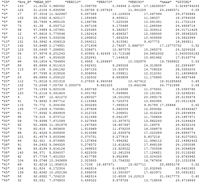
Figure 1: Example of tab-separated input dataset, containing biomass values (response) and remote sensing predictors.

The script will perform a stratified bootstrapping to create 500 bootstraps of the dataset. Additionally the sample size of the input dataset is varied four times (more details can be found in the manuscript mentioned above).

Then the datasets will be fit using 5 different prediction methods (stepwise linear regression, support vector regression, random forest, gaussian processes, knn). Fitting and parameter tuning is accomplished using the "caret" package and a 5-fold cross-validation with 5 repetitions.

Created outputs embrace:

1. RData-files containing the wall-to-wall predictions (based on table 2) of each prediction method and sample size
2. RData-files containing the predicted values calculated during the model building (based on table 1) of each prediction method and sample size
3. RData-files containing the corresponding response values of the model building (based on table 1) of each prediction method and sample size
4. TIFF files showing the summed Residual-Plots of each prediction method and sample size
5. txt-files containing the cross-validated RMSE and r² values of each fitted model. Additionally, standard deviation of RMSE and r² are given, as well as: prediction method, sample size, input data type (sensor), test site, number of folds (k) in the k-fold cross validation

# Step 2 - Prepare ANOVA analysis

R-script named "2_preparation_ANOVA_merge_results.R will merge all txt-files created in step 1. IMPORTANT: Some manual editing required. All .txt files created by "modeling.R" should be copied into one folder. Then the R-script should be run and all .txt files will be added and stored into a single text file.

After merging the textfile a header has to be inserted manually into the first line of the textfile. The header should be (tab-separated):

"RMSE" "R2" "RMSE_SD" "R2_SD" "ExPoMeth" "NumSamp" "InData" "Site" "Folds"

# Step 3 - ANOVA analysis

R-script named "3_anova_analysis.R will calculate the ANOVA and store results to a table.

# Step 4 - calculate plots to have a summary of the obtained RMSE and r² values

R-script named "4_plotresults.R will create beanplots that summarize all results obtained during the model runs. Figure 2 shows a single example of the calculated plots.

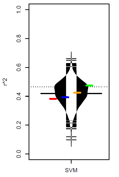
Figure 2: Example of a summarizing result plot.

In Figure 2 the distribution of r² values obtained from the 500 bootrapped datasets fitted with a support vector regression is displayed. The colored horizontal stripes indicate the mean r² values of four applied sample sizes (increasing sample size from left to right). Black horizontal stripe shows overall mean r² value.

# Step 5 - prepare the calculation of wall to wall biomass maps

This step reads the predictions for the full test area as created in Step 1 (from the RData-files). Summary statistics of the 500 bootstraps are calculated and added as an attribute to the fishnet-shapefile, that has originally been used to calculate table 2 (compare Step 1). Again: IMPORTANT: Some manual editing is required. All fullPred_.RData files created by "modeling.R" in Step 1 have to be copied into an own directory. Then the R-code entitled *"5_preparation_biomass_map_plots" can be run.

# Step 6 - calculate wall to wall biomass maps

In the last step the wall-to-wall biomass maps are calculated by using the script "6_biomass_map_plots.R". As input serve the Shapefiles created in Step 5. Figure 3 shows an example of a calculated biomass map.

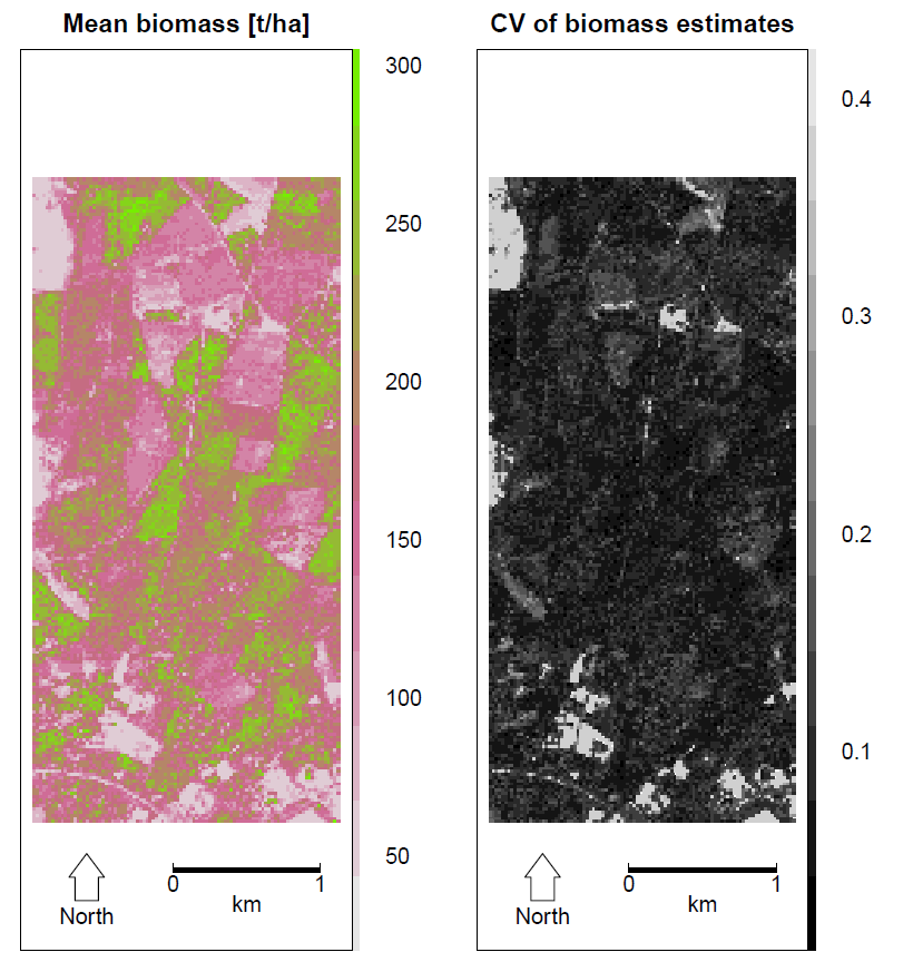
Figure 3: An example of a calculated biomass map.